Building an AI That Plays Rocket League

From scratch, of course

Just like many other developers, I often toggle between building software and playing video games to unwind. A few years ago I came across a project called Python Plays GTA, where the YouTuber built an AI to play Grand Theft Auto V. I wondered if I could do the same in Rocket League, not by manually programming rules or behaviors, but by letting it watch me play and learn by example.

I built a system from scratch that captures both my screen and controller inputs, then trained a neural network to map what's happening on screen to specific controller actions. This article breaks down exactly how I built that system and all the interesting problems I had to solve along the way. All code can be found here, dataset can be found here, and pretrained model can be found here.

The Big Picture: How Does an AI learn to Play Rocket League?

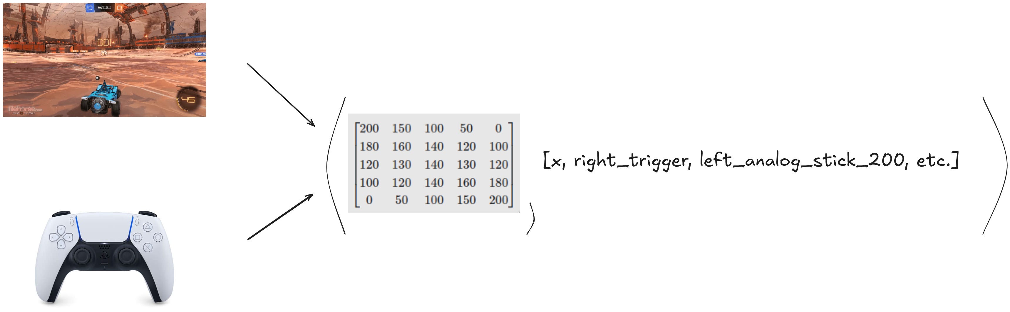
Before we jump into the code, let's understand what we're trying to build at a high level. The goal is to create an AI that can watch Rocket League gameplay and output controller commands (press this button, move this joystick) just like a human player would.

At a high level, here's how the system works:

1. Data Collection: I play Rocket League while my system captures both:

   1. What's happening on my screen (frames from the game)

   2. What I'm doing with the controller (button presses, joystick movements)

2. Training: We feed this data to a neural network that learns to associate what it sees (game frames) with what actions to take (controller inputs).

3. Inference/Evaluation: Once trained, we can feed the AI just the game frames, and it will predict what controller inputs to make, which we then feed back into the game using a virtual controller.

The entire process is what's known as behavioral cloning or imitation learning. The AI is literally learning to imitate my gameplay by watching me play. The project layout is fairly simple:

├── rl_utils/
│   ├── __init__.py
│   ├── apply_inputs.py        # Applies predicted inputs to virtual controller
│   ├── controller_reader.py   # Reads inputs from physical controller
│   ├── data_batcher.py        # Manages saving/loading training data
│   ├── get_current_frame.py   # Captures frames from the game window
│   ├── get_current_window.py  # Monitors the active window
│   └── model.py               # Neural network architecture and loss functions
├── collect.py                 # Script for collecting training data
├── eval.py                    # Script for evaluating the model
├── playback.py                # Script for playing back recorded data
└── train.py                   # Script for training the model

The modular structure made it easier to thing about the different parts of the system.

Part 1: Capturing Training Data

Before our AI can learn anything, we need a dataset showing both what the AI "sees" (game frames) and what it should do (controller inputs). The quality of this dataset will directly impact how well our AI plays. The process needs to be as fast and efficient as possible -- if data collection is too slow or consumes too many resources, it would disrupt gameplay, take an extremely long time to collect, and produce low-quality training data.

What Makes Good Training Data?

Good training data for a Rocket League AI needs:

1. High frame rate - To capture the game's fast pace

2. Diverse gameplay - Different maps, situations, and maneuvers

3. Synchronized inputs - Each frame paired with the exact controller state

4. Efficient storage - Compressed to save disk space without sacrificing quality

Our training data consists of pairs of:

1. Game frames: RGB images of Rocket League gameplay, resized to 270×480 pixels (height, width)

2. Controller inputs: A 19-element vector containing:

   • 11 binary values for button states (0 or 1)

   • 8 analog values for joysticks and triggers (normalized to 0-1)

For reference, here's how the 19 input elements are organized:

BUTTON_CODES = [
ecodes.BTN_SOUTH,
ecodes.BTN_EAST,
ecodes.BTN_NORTH,
ecodes.BTN_WEST,
ecodes.BTN_TL, # Left Bumper
ecodes.BTN_TR, # Right Bumper
ecodes.BTN_SELECT,
ecodes.BTN_START,
ecodes.BTN_MODE,
ecodes.BTN_THUMBL, # Left Stick Press
ecodes.BTN_THUMBR, # Right Stick Press
]

AXIS_CODES = [
ecodes.ABS_X, # Left Stick X
ecodes.ABS_Y, # Left Stick Y
ecodes.ABS_RX, # Right Stick X
ecodes.ABS_RY, # Right Stick Y
ecodes.ABS_Z, # Left Trigger / L2
ecodes.ABS_RZ, # Right Trigger / R2
ecodes.ABS_HAT0X, # D-pad X
ecodes.ABS_HAT0Y, # D-pad Y
]

The D-pad values are technically trinary (-1, 0, 1) rather than analog, but I include them in the analog section for architectural simplicity.

Capturing Game Frames

There are a few considerations when capturing game data:

1. We want to capture it quickly, both so that it doesn't take forever to get enough training samples and to capture the fast pace of Rocket League in high fidelity

2. We need to make sure we capture the whole window and nothing but the window

3. We should only be capturing data when "Rocket League" is the currently active window

In practice, this looks like:

1. Creating a loop

2. Check to see if the current window is "Rocket League"

3. Capture frame/input combo if it is

4. Save to buffer to be written to disk later

The main capture loop can be found here. After several iterations, I landed on using the mss library which offers fast screen captures with minimal overhead. There's a lot going on in the class that capture frames to check for window boundaries, but the key line is this:

frame = np.frombuffer(raw.rgb, dtype=np.uint8).reshape(raw.height, raw.width, 3).copy()

This creates a numpy array directly from the screen buffer into a 1D array, reshapes it into an RGB frame, then copies it to prevent overriding the original data after we perform transforms later on. One big bottleneck I noticed early on was that by reducing the size of the initial screenshot I could speed up the capture rate. I found that by capturing at 1080p and then resizing it down to 480p resulted in faster captures than starting at 1440p or higher.

Note that this implementation uses xdotool, which is Linux-specific. On Windows or Mac, you'd need a different approach to get the window geometry, but the concept remains the same.

Capturing Controller Input

This was actually fairly straightforward. For controller input, I needed to read the state of every button, joystick, and trigger. I used the evdev library to grab raw input events from my PS5 controller:

def get_state_vector(self) -> np.ndarray:
    """Return normalized [buttons..., axes...] vector (19 elements)."""
    # Process any pending events
    try:
        for event in self.device.read():
            if event.type == ecodes.EV_KEY:
                self.button_states[event.code] = event.value
            elif event.type == ecodes.EV_ABS:
                self.axis_states[event.code] = event.value
    except OSError:
        time.sleep(0.1)
    
    # Return normalized vector of inputs
    buttons = np.array([self.button_states.get(code, 0) for code in BUTTON_CODES])
    axes = np.array([self._normalize_axis(code, self.axis_states.get(code, 0)) for code in AXIS_CODES])
    
    return np.concatenate([buttons, axes])

The final output is a 19-element vector:

• First 11 values: Button states (0 or 1)

• Next 6 values: Analog sticks and triggers (normalized from 0 to 1)

• Last 2 values: D-pad (which are technically digital -1/0/1 inputs, but I handle them as analog for consistency)

I normalize these values because neural networks train better on normalized data, helping with gradient flow and convergence.

Efficient Data Storage: Balancing Size and Speed

With 30+ frames per second and each frame needing to be paired with controller inputs, storage efficiency became critical. My first implementation just used numpy arrays dumped to disk, but those files were massive - around 4GB for just 5000 frames!

I solved this by using HDF5 files with gzip compression:

# Save to HDF5 format with compression
filename = os.path.join(self.save_dir, f"{timestamp}_batch.h5")
with h5py.File(filename, "w") as f:
    # Create compressed datasets
    f.create_dataset(
        "frames",
        data=frames_array,
        compression="gzip",
        compression_opts=1,  # Low compression level for speed
    )
    f.create_dataset(
        "inputs",
        data=inputs_array,
        compression="gzip",
        compression_opts=1,
    )

I tested compression levels from 1-9 and found that level 1 achieved great space savings (down to ~1GB per 5000 frames) without adding much CPU overhead.

The data is stored as:

• A 4D array of RGB frames (batch_size x height x width x 3)

• A 2D array of controller inputs (batch_size x 19)

As an aside, I really liked working with h5py. It's such a useful way to work with large datasets. If you are working with large arrays/datasets, consider trying it out.

Background Processing: Preventing Capture Stalls

A big optimization was moving the file saving to a background thread:

# Create copies of current batch data
frames_to_save = self.frames.copy()
inputs_to_save = self.inputs.copy()

# Clear current batch immediately
self.frames.clear()
self.inputs.clear()

# Submit save task to thread pool
def save_task():
    # Conversion and file saving happens here
    
self.executor.submit(save_task)

This was absolutely necessary to prevent the game from freezing during data collection. Without it, the entire computer would lock up every time a batch was saved unless I set the batch size to something unrealistically small.

Putting It All Together: The Data Collection Script

Here's the main loop that ties everything together:

def main() -> None:
    grabber = FrameGrabber()
    controller = ControllerReader()
    batcher = BatchSaver(BATCH_SIZE, SAVE_DIR)
    window_monitor = WindowMonitor()

    try:
        while True:
            if window_monitor.get_active_window() == "Rocket League":
                frame = grabber.capture_frame()
                if frame is None:
                    continue

                inputs = controller.get_state_vector()
                batcher.add_sample(frame, inputs)
                
                # FPS tracking code omitted for brevity
    except KeyboardInterrupt:
        # Save remaining samples
        if batcher.frames:
            batcher._save_batch()

I used this script to collect about an hour's worth of gameplay, generating approximately 150,000 frames of training data.

To verify that the captured data is correct, I created a playback script (playback.py) that:

1. Loads a batch file

2. Displays frames with their corresponding inputs

3. Allows playback at different speeds

This was useful for ensuring that frames and inputs were properly synchronized and that the data quality was high enough for training. Something to note: cv2 loads pixels in bgr format (as opposed to the more standard rgb), so the colors look odd. This does not affect the training data or training process.

Part 2: Building and Training the Model

With a dataset in hand, the next step was to design a neural network capable of learning to map game frames to controller inputs. This wasn't as straightforward as it might seem!

The Challenge of Predicting Mixed Outputs

A key challenge in this project is that the network needs to predict both binary (buttons) and continuous (analog sticks/triggers) values simultaneously. My early experiments with a single-output linear network using MSE as a loss function showed that:

1. The network would easily achieve high accuracy on buttons but struggle with analog controls.

2. A singular feed forward network wasn't able to reliably learn enough about the input frame to reliable predict controller states.

3. A singular feed forward network took up a ton of space in memory -- 300M parameters and nearly 10GB of VRAM!

There were likely other issues with my training loop that were causing the massive amount on in-VRAM memory, but after several iterations I found that using convolutions to reduce the array size and splitting the network into two specialized "heads" – one for binary and one for analog outputs – yielded the best results. Claude 3.7 and R1 were a massive help for this section as it allowed me to explore different ways to optimize my model and training loop much quicker.

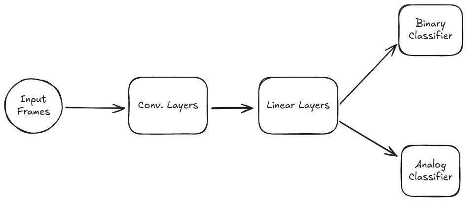
The actual network looks like this:

class RocketNet(nn.Module):
    """Neural network for predicting Rocket League controller inputs from game frames.

    Architecture:
        - Shared convolutional backbone for processing input frames
        - Shared fully connected backbone
        - Separate heads for binary (buttons) and analog (sticks/triggers) outputs
    """

    def __init__(self):
        super(RocketNet, self).__init__()

        # Use convolutional layers to efficiently process the input
        self.conv_backbone = nn.Sequential(
            # First conv block - reduce spatial dimensions
            nn.Conv2d(3, 32, kernel_size=7, stride=4, padding=3),
            nn.ReLU(),
            nn.BatchNorm2d(32),
            nn.MaxPool2d(2),
            # Second conv block - extract features
            nn.Conv2d(32, 64, kernel_size=5, stride=2, padding=2),
            nn.ReLU(),
            nn.BatchNorm2d(64),
            nn.MaxPool2d(2),
            # Third conv block - final feature extraction
            nn.Conv2d(64, 128, kernel_size=3, stride=1, padding=1),
            nn.ReLU(),
            nn.BatchNorm2d(128),
            nn.AdaptiveAvgPool2d((4, 4)),  # Force output to 4x4 spatial dimensions
        )

        # Calculate the flattened size after convolutions (128 * 4 * 4 = 2048)
        self._conv_output_size = 128 * 4 * 4

        # Shared backbone
        self.backbone = nn.Sequential(
            nn.Linear(self._conv_output_size, 512),
            nn.ReLU(),
            nn.BatchNorm1d(512),
            nn.Dropout(0.3),
            nn.Linear(512, 256),
            nn.ReLU(),
            nn.BatchNorm1d(256),
            nn.Dropout(0.2),
            nn.Linear(256, 128),
            nn.ReLU(),
        )

        # Binary controls (buttons) - no activation
        self.binary_head = nn.Linear(128, 11)

        # Improved analog head with more expressive architecture
        self.analog_head = nn.Sequential(
            nn.Linear(128, 64),
            nn.LayerNorm(64),  # Normalize activations
            nn.LeakyReLU(0.1),
            nn.Dropout(0.1),  # Prevent overfitting
            nn.Linear(64, 8),
            nn.Sigmoid(),
        )

        # Apply weight initialization
        self._initialize_weights()

We'll get to _initialize_weights() in a bit, there are some design choices I'd like to explain first. The first is that in order to reduce the size of the network, we need to rapidly and aggressively reduce the dimension sizes of the input batch:

nn.Conv2d(3, 32, kernel_size=7, stride=4, padding=3)

The 7x7 kernel captures broad visual elements (car shapes, field lines, ball), stride 4 rapidly reduces dimensions (4x smaller in each dimension), and padding 3 preserves edge information (important for seeing goals/walls). This animation of how convolutions work may help convey the concept easier.

After that we perform a standard ReLU activation, then nn.BatchNorm2d(32). This helps to stabilize early feature detection by standardizing activation ranges, preventing any single visual feature (like the ball) from dominating.

From there we use nn.MaxPool2d(2) to take only the most prominent features and further reduce computation by 4x.

This process repeats twice more, extracting more features at finer and finer levels of detail, until we get to the end where we have nn.AdaptiveAvgPool2d((4, 4)). This makes sure to force the final output to be the correct dimension to send into the linear layer, no matter the size of our input image, should we choose to change it in the future. This lets us easily experiment with different resolutions without needed to reconfigure our network.

From there we can move on to the linear layers. When processing the 2048 flattened features from the convolutional backbone, some neurons might detect highly specific game elements (e.g., "ball on wall" or "car in air") that activate strongly only in certain situations. nn.BatchNorm1d(512) prevents these specialized neurons from dominating the representation, giving equal importance to all detected features.

The same logic applies to the second BatchNorm1d, but at a higher abstraction level. We don't add a third normalization layer after the last linear layer because it allows more diverse activation patterns for the separate heads.

Now, onto the heads:

# Binary controls (buttons) - no activation
self.binary_head = nn.Linear(128, 11)

# Improved analog head with more expressive architecture
self.analog_head = nn.Sequential(
    nn.Linear(128, 64),
    nn.LayerNorm(64),  # Normalize activations
    nn.LeakyReLU(0.1),
    nn.Dropout(0.1),  # Prevent overfitting
    nn.Linear(64, 8),
    nn.Sigmoid(),
)

Originally I just had a single linear layer for both heads, but I found that the analog heads were not really learning, so I added a few more layers and a nn.LayerNorm(64). When predicting analog controls for a Rocket League controller, the relationship between different controls is important (e.g., coordinating throttle, steering, and boost). LayerNorm maintains these relationships within each sample, making predictions more coherent.

After the layer norm we see the first and only instance of nn.LeakyReLU. The idea is that regular ReLU might cause "dead" neurons for rarely-used control combinations. LeakyReLU ensures the network can maintain sensitivity to subtle analog stick movements, recover when learning rare but important control patterns (air rolls, flip resets), and prevent gradients from becoming zero during backpropagation. If using ReLU, certain control patterns might never be learned if they initially produce negative values. LeakyReLU with α=0.1 allows a small gradient flow even when the neuron is not activated, maintaining learning capacity for all control possibilities.

At a super high level, there is a theme of stabilization early on in the network that gives way to more creative and diverse outcomes later on. The decreasing value for the various dropout layers reflects that, progressively letting more and more neurons have a say in the final output.

Initializing Weights

Now that we've defined the network, let's address the _initialize_weights() call:

def _initialize_weights(self):
    for m in self.modules():
        if isinstance(m, (nn.Linear, nn.Conv2d)):
            nn.init.kaiming_normal_(m.weight, mode="fan_out", nonlinearity="relu")
            if m.bias is not None:
                nn.init.constant_(m.bias, 0)
        elif isinstance(m, (nn.BatchNorm1d, nn.BatchNorm2d)):
            nn.init.constant_(m.weight, 1)
            nn.init.constant_(m.bias, 0)

By default, PyTorch initializes weights with small random values. This seems reasonable but leads to major issues in deep networks:

• In deep networks, these random values compound across layers

• With ReLU activations, roughly half of neurons become inactive immediately (any negative input results in zero output)

• Signal strength either explodes or vanishes entirely by the time it reaches deep layers

• The result? Training either fails completely or takes an excessively long time

Early in my experiments with random initialization, the network struggled to learn even basic patterns, with loss values stubbornly refusing to decrease. While I can’t directly attribute the high loss value to the random initialization, I know that after I added kaiming initialization I was able to achieve a lower loss value.

The core concept behind good initialization is "preserving variance" across layers. Think of it like this: we want the signal strength to remain relatively consistent as it passes through each layer of the network.

With standard random initialization, each layer changes the statistical properties of the signal:

• Too small → signal fades away (vanishing gradient)

• Too large → signal explodes (exploding gradient)

Kaiming initialization (kaiming_normal_) solves this by calculating the variance based on the number of connections in the layer. For a layer with n inputs, it uses a variance of 2/n for ReLU networks. I use mode="fan_out" with Kaiming initialization, which preserves the magnitudes in the backwards pass. This choice prioritizes stable gradient flow during backpropagation, which is particularly important for our deep network to learn effectively. Unlike fan_in (which stabilizes forward propagation), fan_out helps ensure gradients don't vanish or explode when flowing backward through the network during training.

Each layer type needs different initialization:

1. For Convolutional and Linear Layers: Standard random initialization would produce signals that are either too weak or too strong. Kaiming initialization creates a statistical "sweet spot" specifically calibrated for ReLU activations, keeping signals in the optimal range.

2. For Bias Parameters: Random bias values would introduce unnecessary initial offsets. Zero initialization provides a clean starting point, letting the network focus on learning meaningful patterns from data rather than overcoming random biases.

3. For Batch Normalization Layers: The default random initialization would immediately distort the normalized signals. Setting weights to 1 and biases to 0 ensures batch normalization initially performs pure standardization, letting the network learn any necessary adjustments gradually.

For Rocket League specifically, proper initialization makes a huge difference because our network needs to learn subtle control adjustments while also recognizing dramatic game state changes.

Custom Loss Function

Let's break down our custom loss function, which is specially designed to handle for the split head approach of our model:

def compute_improved_loss(outputs: torch.Tensor, targets: torch.Tensor) -> torch.Tensor:
    # Split the outputs and targets
    binary_logits = outputs[:, :11]  # First 11 are binary controls
    analog_values = outputs[:, 11:]  # Last 8 are analog controls

    binary_targets = targets[:, :11]
    analog_targets = targets[:, 11:]

    # Add epsilon for numerical stability
    eps = 1e-7

    # Use focal loss for binary controls
    focal_loss = FocalLoss(gamma=2.0, alpha=0.25)
    binary_loss = focal_loss(binary_logits, binary_targets)

    # Ensure analog values are in valid range
    analog_values = torch.clamp(analog_values, eps, 1.0 - eps)

    # Use smooth L1 loss for analog controls
    analog_loss = F.smooth_l1_loss(analog_values, analog_targets, reduction="mean", beta=0.1)

    # Add distribution regularization for analog outputs
    analog_distribution_loss = 0.0
    if analog_values.size(0) > 1:  # Only if batch size > 1
        # Encourage diversity in predictions across the batch
        analog_std = torch.clamp(analog_values.std(dim=0, unbiased=False), min=0.1)
        analog_distribution_loss = 0.05 * (1.0 / analog_std).mean()

    # Total loss with increased analog weight and distribution regularization
    total_loss = binary_loss + 3.0 * analog_loss + analog_distribution_loss

    # Final safety check
    if torch.isnan(total_loss) or torch.isinf(total_loss):
        return torch.tensor(0.1, device=total_loss.device, requires_grad=True)

    return total_loss

Standard neural networks typically optimize for a single type of output - either classification or regression. Our controller model needs to handle both simultaneously:

1. Binary controls: 11 buttons that are either pressed or not pressed

2. Analog controls: 8 joystick/trigger values that range continuously from 0 to 1

My first attempts with a single loss function like Mean Squared Error performed poorly - the network learned to predict buttons reasonably well but struggled with analog sticks. I believe this occurred because binary predictions are computationally simpler to optimize, so the network focused on those at the expense of the more challenging analog predictions.

To fix it, for buttons, I implemented Focal Loss - a specialized version of binary cross-entropy that gives more weight to difficult examples:

class FocalLoss(nn.Module):
    def __init__(self, gamma=2.0, alpha=0.25):
        super(FocalLoss, self).__init__()
        self.gamma = gamma
        self.alpha = alpha

    def forward(self, logits: torch.Tensor, targets: torch.Tensor) -> torch.Tensor:
        # Apply sigmoid to get probabilities
        probs = torch.sigmoid(logits)

        # Get the binary cross entropy loss
        bce_loss = F.binary_cross_entropy_with_logits(logits, targets, reduction="none")

        # Calculate focal weights
        p_t = probs * targets + (1 - probs) * (1 - targets)
        alpha_t = self.alpha * targets + (1 - self.alpha) * (1 - targets)
        focal_weight = alpha_t * (1 - p_t) ** self.gamma

        # Apply weights to BCE loss
        loss = focal_weight * bce_loss

        return loss.mean()

There's a lot going on there, but in short focal loss addresses class imbalance in the button data - most buttons remain unpressed during the majority of gameplay. The alpha parameter gives more weight to the less common class, while the gamma parameter focuses training on harder examples where predictions are far from targets.

For joysticks and triggers, I use Smooth L1 Loss:

analog_loss = F.smooth_l1_loss(analog_values, analog_targets, reduction="mean", beta=0.1)

Smooth L1 combines the benefits of both MSE and MAE:

• Like MSE (Mean Squared Error), it strongly penalizes large errors

• Like MAE (Mean Absolute Error), it's less sensitive to outliers

• The small beta value (0.1) creates sharper transitions between the L1 and L2 regions

This helps the network make precise analog predictions while remaining robust to occasional outliers in the training data.

# Add distribution regularization for analog outputs
analog_distribution_loss = 0.0
if analog_values.size(0) > 1:  # Only if batch size > 1
    # Encourage diversity in predictions across the batch
    analog_std = torch.clamp(analog_values.std(dim=0, unbiased=False), min=0.1)
    analog_distribution_loss = 0.05 * (1.0 / analog_std).mean()

Early versions of the network would "play it safe" by predicting middle values for analog controls, rather than committing to extreme values. This "regression to the mean" is a common problem in neural networks trained on imitation learning tasks. I discovered that without specific countermeasures, the model would consistently predict joystick and trigger values clustered tightly around 0.5 (neutral position).

What was happening is a phenomenon called "distribution collapse" - instead of learning the full range of possible actions, the network was converging toward the statistical average of the training data. This makes mathematical sense from the network's perspective: predicting values around 0.5 minimizes average error across all scenarios, even though these "safe" predictions are rarely optimal for any specific gameplay moment. The Smooth L1 loss function I was using actually compounded this problem, as it inherently penalizes extreme predictions more heavily when they're wrong, making the network hesitant to predict values near 0 or 1.

In Rocket League terms, this manifested as an AI that barely turned the steering wheel, rarely committed to full boost or brake, and made half-hearted jumps and aerials. In situations where human players would slam the stick to one extreme for a sharp turn or powerslide, the AI would make timid adjustments, missing the ball or failing to recover from awkward positions.

To solve this, I implemented the distribution regularization term shown above. This code measures the standard deviation of predicted values across each batch for each analog control, with torch.clamp() ensuring a minimum threshold of 0.1 to prevent numerical instability. The inverse relationship (1.0 / analog_std) creates an exponentially increasing penalty as predictions become more similar. When the network starts predicting nearly identical analog values across different situations, this regularization term spikes, forcing it to reconsider.

What makes this particularly effective is that it encourages the network to match not just the expected value of human actions but their statistical variance as well. By computing std(dim=0), I measure diversity separately for each analog control, preventing the model from satisfying the regularization by varying only one control while keeping others uniform. The small coefficient of 0.05 carefully weights this regularization to guide rather than dominate the learning process.

The impact on gameplay was dramatic. With regularization, the model began making bold, decisive movements that much better mimicked human play patterns – full boost when racing for the ball, hard turns for positioning, committed jumps for aerials, and rapid directional changes when dribbling. It represents a form of "behavioral prior" that encodes the human tendency toward decisive action in high-speed competitive games, something conventional supervised learning alone failed to capture.

After experimentation, I found that weighing analog loss by ~3x was useful for balancing the learning rate:

total_loss = binary_loss + 3.0 * analog_loss + analog_distribution_loss

This prevents the network from focusing too much on button accuracy at the expense of analog precision. In practice this allowed the analog loss to almost keep pace with the binary loss.

After experimentation, I found that weighing analog loss by ~3x was useful for balancing the learning rate:

total_loss = binary_loss + 3.0 * analog_loss + analog_distribution_loss

This prevents the network from focusing too much on button accuracy at the expense of analog precision. In practice this allowed the analog loss to almost keep pace with the binary loss.

Training Loop: How the AI Actually Learns

Now comes the interesting part - watching the neural network gradually learn to mimic my gameplay. This training process evolved through several iterations, with each version improving on accuracy, efficiency, and stability. Let me walk you through how I approached it.

Setting Up the Training Environment

Before diving into the training loop itself, I prepared the environment to help ensure the process would be stable, reproducible, and efficient:

torch.multiprocessing.set_sharing_strategy("file_system")

This line sets how PyTorch shares tensor data between processes. According to the PyTorch documentation, there are two main strategies: file_descriptor (the default on most systems) and file_system. The file_system strategy uses filenames to identify shared memory regions rather than keeping file descriptors open. While this approach can be prone to memory leaks if processes crash abruptly, PyTorch mitigates this by using a daemon process called torch_shm_manager to track and clean up shared memory allocations. I chose this strategy because at one point early on while building this I was running into erroneous issues with accessing my files. Furthermore, it avoids issues with systems that have low limits on the number of open file descriptors, which can become a problem when processing large datasets with many parallel workers.

For reproducibility and debugging, I set fixed random seeds:

# Set random seed for reproducibility
random.seed(42)
np.random.seed(42)
torch.manual_seed(42)
if torch.cuda.is_available():
    torch.cuda.manual_seed(42)
    torch.backends.cudnn.deterministic = True
    torch.backends.cudnn.benchmark = False

This code explicitly prioritizes reproducibility over speed. When torch.backends.cudnn.benchmark is set to True, PyTorch conducts an exhaustive search at startup to find the optimal cuDNN algorithm for each convolutional layer in the network. This can significantly accelerate training (potentially by 15% or more), but introduces variability in results.

By keeping benchmark=False and setting deterministic=True, PyTorch uses consistent, deterministic algorithms instead. This ensures that given the same inputs, the network produces identical outputs across different runs, which is invaluable for debugging and development. The slight performance cost is worthwhile during the model development phase, where consistency matters more than raw speed.

For efficient data loading and processing of the dataset of gameplay videos, I configured the DataLoader with these settings:

# DataLoader configuration
dataloader_kwargs = {
    "batch_size": batch_size,
    "shuffle": True,
    "pin_memory": True,
    "num_workers": 4,
    "persistent_workers": False,
}

Each setting serves a specific purpose:

• shuffle=True randomizes training data to prevent the model from learning sequence-dependent patterns

• pin_memory=True speeds up GPU transfers by using pinned CPU memory

• num_workers=4 enables parallel data loading with 4 processes

• persistent_workers=False shuts down worker processes after each epoch to free up resources

I use this configuration for the training data loader:

train_loader = DataLoader(train_dataset, **dataloader_kwargs)

For validation, I created a separate loader with different parameters:

val_loader = DataLoader(val_dataset, batch_size=batch_size * 2, pin_memory=True)

The validation loader uses twice the batch size since validation doesn't need gradient calculations (which use significant GPU memory). I skipped the multi-worker setup for validation as it's less impactful for overall performance.

The Challenge of Training a Mixed-Output Network

With the architecture and loss function in place, I implemented a training loop with specific considerations for Rocket League's fast-paced gameplay:

# Training loop
training_start_time = time()
for epoch in range(epochs):
    epoch_start_time = time()
    print(f"\nEpoch {epoch + 1}/{epochs}")
    print("-" * 50)

    # Shuffle h5 files for each epoch
    np.random.shuffle(h5_files)

    model.train()
    epoch_loss = 0
    batch_count = 0
    total_val_loss = 0
    total_val_batches = 0

I process files one by one rather than loading everything into memory at once. This "batch generator" approach works well since the full dataset would be too large to fit in RAM:

# Process each file
for file_idx, (
    h5_file,
    (train_frames, train_inputs, val_frames, val_inputs),
) in enumerate(batch_generator(h5_files)):
    file_start_time = time()
    n_samples = len(train_frames) + len(val_frames)
    files_processed += 1

For each file, I split the data into training and validation sets, with 80% used for training. This per-file validation provides feedback on how well the model generalizes to unseen data within the same gameplay session.

Mixed Precision

In my early implementation attempts, I experimented with mixed precision training:

# This code was ultimately not used in the final implementation
from torch.cuda.amp import autocast, GradScaler

# Initialize scaler for mixed precision training
scaler = GradScaler()

# In training loop:
with autocast(device_type='cuda', dtype=torch.float16):
    # Forward pass would run in FP16 where beneficial
    outputs = model(batch_X)
    loss = compute_improved_loss(outputs, batch_y)

# Scale loss and run backward pass
scaler.scale(loss).backward()
scaler.step(optimizer)
scaler.update()

There's a drawback with using mixed precision on my GTX 1080 Ti: the card has limited FP16 support. While newer GPUs have specialized Tensor Cores that accelerate FP16 operations, the 1080 Ti's FP16 throughput is only about 177 GFLOPS compared to its 11.3 TFLOPS FP32 performance, or about 1/64 the speed.

I removed the mixed precision components for two reasons:

1. No performance benefit: Without proper hardware support, mixed precision would actually slow training down.

2. Memory wasn't a bottleneck: With the other optimizations in the training pipeline, the model used only a couple GB of VRAM during training - well within the 11GB available on the 1080 Ti.

There are some leftover artifacts from the mixed precision experiments in the code:

../
└── train.py
Code:
   205 | scaler = GradScaler()  # For mixed precision training
   ...
   368 |             scaler.scale(loss).backward()
   ...
   388 |                 scaler.unscale_(optim)
   ...
   420 |                 scaler.step(optim)
   421 |                 scaler.update()

I left them in since they don't affect functionality, though a cleaner implementation would be to remove them.

Balancing Head Gradients

I noticed that the binary head learned much faster than the analog head, which makes sense - predicting button presses is simpler than predicting exact joystick positions.

I implemented gradient balancing to address this imbalance:

# Get average gradient magnitudes for each head
binary_grad_norm = torch.norm(
    torch.stack(
        [
            torch.norm(p.grad)
            for p in model.binary_head.parameters()
            if p.grad is not None
        ]
    )
)
analog_grad_norm = torch.norm(
    torch.stack(
        [
            torch.norm(p.grad)
            for p in model.analog_head.parameters()
            if p.grad is not None
        ]
    )
)

# If binary gradients dominate, scale them down
if binary_grad_norm > 2.0 * analog_grad_norm:
    scale_factor = analog_grad_norm / binary_grad_norm
    for p in model.binary_head.parameters():
        if p.grad is not None:
            p.grad *= scale_factor

This code checks if binary gradients are more than twice as strong as analog gradients. If so, it scales them down to give the analog head more influence in learning.

Without this balancing, the model would become good at pressing buttons but poor with analog controls. In my early experiments before adding this code, the binary accuracy would reach ~90% while analog accuracy stayed below 60%. After implementing gradient balancing, the analog accuracy improved to around 80%.

In evaluation tests, this improvement resulted in better driving and steering behavior.

Regularization and Robustness: Fixing Unstable Training

Training neural networks can be unstable, especially for tasks like Rocket League control where the network makes both binary and continuous predictions. Early versions of my training loop would sometimes produce large loss spikes or NaN values. I added checks for these problems throughout the training process:

# Skip if NaN/Inf outputs detected
if torch.isnan(outputs).any() or torch.isinf(outputs).any():
    print(f"NaN/Inf in outputs detected at batch {batch_count}. Skipping batch.")
    continue

# Calculate loss with improved loss function
loss = compute_improved_loss(outputs, batch_y)
loss = loss / accumulation_steps

# Skip if NaN loss
if torch.isnan(loss):
    print(f"NaN loss detected at batch {batch_count}. Skipping batch.")
    continue

These checks prevent a problematic batch from derailing the entire training process. I also added gradient clipping:

# Apply normal gradient clipping
torch.nn.utils.clip_grad_norm_(model.parameters(), max_grad_norm)

By limiting gradient magnitudes to max_grad_norm (in my case, 1.0), the model avoids large parameter changes that can cause instability. This helps in deep networks where gradients can grow very large during backpropagation.

These safeguards not only prevented crashes but also helped the model learn more consistently.

Metrics Tracking

To track progress beyond just the loss value, I added metrics for both binary and analog predictions:

def calculate_metrics(
    outputs: torch.Tensor, targets: torch.Tensor
) -> tuple[float, float, float, float]:
    # Split the outputs
    binary_logits = outputs[:, :11]
    analog_values = outputs[:, 11:]

    # Split the targets
    binary_targets = targets[:, :11]
    analog_targets = targets[:, 11:]

    # Binary metrics
    binary_probs = torch.sigmoid(binary_logits)
    binary_preds = (binary_probs >= 0.5).float()
    binary_accuracy = (binary_preds == binary_targets).float().mean().item()

    # Analog metrics with multiple thresholds
    analog_errors = torch.abs(analog_values - analog_targets)
    analog_strict = (analog_errors < 0.01).float().mean().item()  # Within 1%
    analog_usable = (analog_errors < 0.05).float().mean().item()  # Within 5%

    # Use the usable metric for training feedback while tracking strict
    analog_accuracy = analog_usable

    # Calculate combined accuracy
    combined_accuracy = (binary_accuracy + analog_accuracy) / 2

    return binary_accuracy, analog_accuracy, combined_accuracy, analog_strict

This is called after each file is trained:

            # Calculate and track metrics
            with torch.no_grad():
                binary_acc, analog_acc, combined_acc, analog_strict = calculate_metrics(
                    outputs, batch_y
                )

For analog controls, I track two thresholds:

• Strict (1%): Controls within 1% of the target value

• Usable (5%): Controls within 5% of the target value

For context, with a joystick range of -1.0 to 1.0, a 1% error means being off by only 0.02 in either direction - hardly noticeable in gameplay. A 5% error (being off by 0.1) still results in playable controls. Even human players don't consistently use exact analog values.

I visualized these metrics in TensorBoard to monitor training progress:

# Log training metrics to tensorboard
if i % 5 == 0 or i + 1 == len(train_loader):
    global_step = epoch * len(h5_files) * len(train_loader) + batch_count
    writer.add_scalar("Training/Loss", loss.item() * accumulation_steps, global_step)
    writer.add_scalar("Training/Learning_Rate", scheduler.get_last_lr()[0], global_step)
    writer.add_scalar("Training/Binary_Accuracy", binary_acc, global_step)
    writer.add_scalar("Training/Analog_Accuracy", analog_acc, global_step)

These visualizations helped identify plateaus and regressions during training. For example, I observed that analog accuracy would sometimes decrease when the model improved its binary predictions - a side effect of the competition between heads that led me to implement gradient balancing.

Learning Rate Scheduling: Finding the Sweet Spot

Finding an effective learning rate takes experimentation - too high and training becomes unstable, too low and progress is slow. After trying constant rates, step schedules, and exponential decay, I settled on OneCycleLR scheduling:

# OneCycleLR scheduler
scheduler = torch.optim.lr_scheduler.OneCycleLR(
    optim,
    max_lr=3e-4,
    total_steps=total_steps,
    pct_start=0.3,
    div_factor=25,
    final_div_factor=1000,
)

The OneCycleLR scheduler follows this pattern:

1. Start with a low learning rate (1.2e-5 in my case, calculated as max_lr/div_factor)

2. Gradually increase to the maximum learning rate (3e-4) during the first 30% of training

3. Slowly decrease to a very small value (3e-7) by the end of training

The learning rate curve in TensorBoard shows this pattern clearly:

This approach has several benefits:

1. Faster convergence: The increasing learning rate helps escape local minima early in training

2. Better generalization: The decreasing phase helps fine-tune the model without overfitting

3. Less manual tuning: It automatically adjusts the learning rate, reducing the need for extensive hyperparameter testing

In my experiments, OneCycleLR performed better than fixed learning rates. With a constant rate of 1e-4, the model would either converge too slowly or wouldn't reach a good loss value, even with momentum. With OneCycleLR, training was faster and the final model performed better at inference time.

Early Stopping

Neural networks can overfit with too much training. To prevent this, I added early stopping that monitors validation loss and stops when it stops improving:

# Early stopping configuration
early_stopping = {
    "best_val_loss": float("inf"),
    "patience": 5,
    "counter": 0,
    "best_epoch": 0,
}
...
# Early stopping check
if avg_val_loss < early_stopping["best_val_loss"]:
    early_stopping["best_val_loss"] = avg_val_loss
    early_stopping["counter"] = 0
    early_stopping["best_epoch"] = epoch + 1

    # Save best model separately
    torch.save(model.state_dict(), "rlai-1.4M/rlai-1.4M.pth")
    print("✓ Saved new best model with validation loss: {:.4f}".format(avg_val_loss))
else:
    early_stopping["counter"] = float(early_stopping["counter"] + 1)
    print(
        "! Validation loss did not improve for {} epochs. Best: {:.4f} at epoch {}".format(
            early_stopping["counter"],
            early_stopping["best_val_loss"],
            early_stopping["best_epoch"],
        )
    )

    if early_stopping["counter"] >= early_stopping["patience"]:
        print("⚠ Early stopping triggered after {} epochs".format(epoch + 1))
        break

The patience parameter (5 epochs) allows the model to work through temporary plateaus before stopping.

Memory Management

Training deep neural networks on high-resolution images can use a lot of GPU memory. Several early training runs crashed from out-of-memory errors, so I implemented memory optimization techniques:

1. Batch size tuning: Started with a batch size of 128

2. Gradient accumulation: Simulates larger batches (effectively 512) without the memory cost by accumulating gradients over multiple smaller batches

3. Per-file processing: Loading one data file at a time instead of the entire dataset

4. Memory monitoring: Tracking GPU memory usage to identify potential issues

# Log memory usage
memory_allocated = torch.cuda.memory_allocated(device) / 1024**3  # To GB
memory_reserved = torch.cuda.memory_reserved(device) / 1024**3  # To GB
writer.add_scalar("System/GPU_Memory_Allocated_GB", memory_allocated, file_step)
writer.add_scalar("System/GPU_Memory_Reserved_GB", memory_reserved, file_step)

This monitoring helped identify memory leaks and optimize the training pipeline. Early versions would gradually consume more memory until they crashed.

Part 3: Evals/Inference

The core of our evaluation process is a simple but effective inference loop that connects our trained model to the game. After spending significant time on data collection and training, this is where our AI finally gets to play the game. At a high level, our inference pipeline works like this:

1. Capture frames from the active Rocket League window

2. Process these frames to match our model's expected input format

3. Run inference through our trained neural network

4. Convert predictions to controller inputs

5. Apply these inputs to a virtual controller that controls the game

This creates a continuous loop that allows the AI to play the game just like a human would - by seeing what's happening on screen and responding with appropriate controller inputs.

Building the Inference Pipeline

The inference pipeline is straightforward in concept but requires careful implementation to work smoothly:

model = RocketNet()
model.load_state_dict(torch.load("rlai-1.4M/rlai-1.4M.pth"))
model.eval()
device = "cuda"
model.to(device)

def main() -> None:
    """Run the AI evaluation process."""
    grabber = FrameGrabber()  # Captures frames from the game
    window_monitor = WindowMonitor()  # Monitors active window
    input_applier = InputApplier(debug_mode=True)  # Applies inputs to virtual controller
    
    target_size = (480, 270)  # Same size used during training
    
    print("Ready to play Rocket League! Focus window to begin...")
    
    try:
        with torch.no_grad():  # Disable gradient tracking for inference efficiency
            while True:
                if window_monitor.get_active_window() == "Rocket League":
                    # Capture frame
                    frame = grabber.capture_frame()
                    if frame is None:
                        continue
                        
                    # Preprocess
                    frame = cv2.resize(frame, target_size)
                    frame = torch.Tensor([frame]).to(device)
                    
                    # Run inference
                    output = model(frame)
                    
                    # Apply to virtual controller
                    input_applier.apply_inputs(output)
                    
    except KeyboardInterrupt:
        print("\nStopping inference/evals.")
    finally:
        input_applier.close()  # Clean up the virtual controller

This loop runs continuously, processing around 30 frames per second to match the pace of gameplay. The key to making this work is ensuring each step runs efficiently, so after a quick resizing of the frame we immediately shuttle it off to the GPU to be processed. From there we perform an inference of a single frame, get the logits, then pass the logits directly into the input_applier

Connecting to a Virtual Controller

The most interesting and challenging part is translating our model's outputs into actual controller inputs. For this, we created the InputApplier class which manages a virtual controller via the evdev library:

def apply_inputs(self, predictions: torch.Tensor | np.ndarray) -> None:
    """Apply the neural network predictions to the virtual controller."""
    # Convert predictions to numpy if needed
    if isinstance(predictions, torch.Tensor):
        predictions = predictions.detach().cpu().numpy()
    
    if predictions.ndim == 2:
        predictions = predictions.squeeze(0)
        
    # Process button inputs (first 11 values)
    for code, value in zip(button_codes, predictions[:11]):
        button_state = int(value > 0.5)  # Simple threshold for buttons
        self.ui.write(ecodes.EV_KEY, code, button_state)
    
    # Process analog inputs (next 6 values for sticks/triggers)
    stick_trigger_values = predictions[11:17]
    scaled_values = np.zeros_like(stick_trigger_values)
    
    # Process joystick axes (first 4 values)
    for i in [0, 1, 2, 3]:  # Stick axes
        # Center around 0.5 (neutral)
        centered_value = stick_trigger_values[i] - 0.5
        
        deadzone = 0.025  # 2.5% deadzone for all stick movement
        sensitivity = 1.0  # Base sensitivity
        
        # Apply deadzone
        if abs(centered_value) < deadzone:
            scaled_values[i] = 128  # Center position
        else:
            # Apply sensitivity adjustments
            adjusted_value = centered_value * sensitivity
            base_scaled = (adjusted_value + 0.5) * 255
            
            # Different scaling for different sticks
            if i in [0, 1]:  # Left stick (movement)
                scaled_values[i] = np.clip(base_scaled * 2, 0, 255)
            else:  # Right stick (camera)
                scaled_values[i] = np.clip(base_scaled / 2, 0, 255)
    
    # Process triggers (last 2 values)
    scaled_values[4:6] = np.clip(stick_trigger_values[4:6] * 255, 0, 255)
    
    # Apply all analog values
    for code, value in zip(analog_codes, analog_values):
        self.ui.write(ecodes.EV_ABS, code, int(value))
        
    # Sync all events to ensure they're applied together
    self.ui.syn()

Several important transformations happen in this code:

1. Thresholding button inputs: We convert continuous values to binary using a threshold of 0.5. This might be leftover from some prior experimentation, but it worked so I left it in.

2. Deadzone application: A small deadzone (2.5%) around the center position prevents jittery stick movement when the model outputs values near neutral

3. Different scaling for different controls: I apply different scaling factors to the left stick (movement) and right stick (camera). This was to address a weird behavior where the model would predict extreme values - the right stick would always max out at 255, while the left stick struggled to go above 128. I'm still not sure why this happened, but this adjustment fixed it.

4. Synchronous event application: The ui.syn() call ensures all inputs are applied together, mimicking how a human would coordinate multiple simultaneous actions

Debugging with Visual Feedback

During development, I added printing of controller states to help debug the model's behavior:

# Print final commands
print("\nFinal controller commands:")
print("Button States:")
for code, value in zip(button_codes, predictions[:11]):
    button_state = int(value > 0.7)
    print(f"  {ecodes.BTN[code]}: {'Pressed' if button_state else 'Released'}")

print("\nAnalog Values:")
analog_names = ["Left Stick X", "Left Stick Y", "Right Stick X", "Right Stick Y", 
                "Left Trigger", "Right Trigger"]
for name, value in zip(analog_names, scaled_values):
    print(f"  {name}: {int(value)}")

This visual feedback was invaluable for understanding what the model was actually doing. Often, the model would produce outputs that seemed reasonable in isolation but created strange behavior when combined. For example, pressing boost while rapidly oscillating the steering would cause the car to lose control—something a human player would rarely do.

Unexpected AI Behaviors

The AI occasionally exhibited behaviors that were quite surprising. If I kept the controller plugged in when I ran inference on the model, sometimes the game would detect two controllers and activate split-screen mode, completely changing how the game frames looked compared to the training data. Other times, the virtual controller took control of my keyboard and started pressing buttons erratically, causing me to reboot it. This happened because the model occasionally triggered combinations of inputs that would activate system hotkeys. For instance, pressing Alt+Tab would switch windows, and once the window focus changed from Rocket League, the model's predictions became completely inappropriate for the new context.

Watching it play

At the end of all that, we get this video:

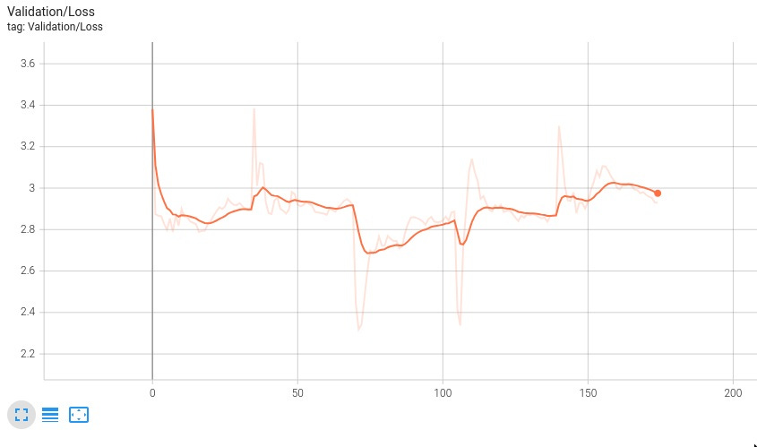
And if you like pretty graphs, here’s the final training state:

While it may not look impressive at first glance, you can see the car actually driving towards the ball at times. It's boosting, seeking out boost pads, jumping, flipping, and even self-correcting in mid-air! What's particularly noteworthy is that this behavior emerged despite training across randomized maps, with inconsistent team colors, and limited recording coverage. The model would likely perform substantially better if trained on a single map with consistent team assignment - but even with these constraints, it's demonstrating fundamental Rocket League mechanics and decision-making.

---

And with that, I hope you enjoyed the ride and learned something useful. As a reminder, everything posted here is open source. All code can be found here, dataset can be found here, and pretrained model can be found here.